Short-term traffic flow forecasting
Short-term traffic flow forecasting (STFF) is an essential aspect of intelligent transportation systems (ITS). Even though auto-regressive moving average (ARMA) has been widely used as one of the most precise methods in such a problem, it has several weaknesses.
In this work, a spatial temporal model is proposed and the joint forecast is performed on the traffic flow and the vehicle number of the link. Using an additional variable, vehicle number, allows better forecasts, and adaption to the dynamic traffic scenarios. Applying this model on an expanded traffic network enables the prediction of spatial effects, from one source to another. Real-time prediction might be obtained by parallel and independent inference on separate links and junctions.
ARMA
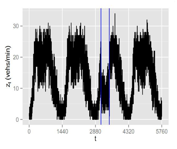
A 4-day simulated traffic flow of 1-minute data collection interval with a traffic accident at time index 3100 is pictured. Several weaknesses of ARMA limit its usage in traffic flow, according to the images. The model adapts slowly to the dynamic situation with he multi-step prediction suffering from exponential decay.
The intractability of moving average, and the non-parallelisable inference make multivariate ARMA impractical, and not scalable to a large traffic network.

Traffic Networks and the General Model
4-day data with a traffic blocking incident is obtained from transportation micro-simulator VISSIM with the below network map. The dataset consists of link in-flows z1,t and out-flows z2,t and the vehicle numbers, vt of all directed links
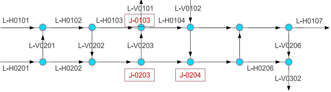
The general model consists of 4 sub-models
- The root link: z1,t=frlk(z1,t-1)
- The link: z2,t=flk(vt-1,z1,t-1)
- The junction: ζ2,t=fjc(ζ1,t) where ζ1,t,ζ2,t are junction inflows and outflows
- The occupancy: vt=fo(vt-1,z2,t-1,z1,t-1)
The Link Sub-Model
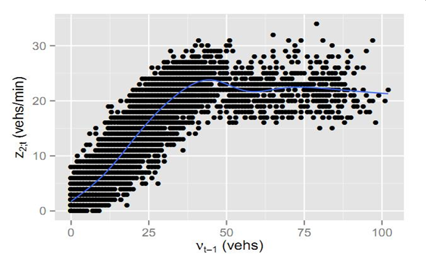
Piecewise polynomial smoothing is used for the link module. In the analysis of 1-minute dataset, the effect of z1,t-1 to z2,t seems negligible. One possible candidate model is:
y=xΒ0+(x-k1)+Β1+(x-k2)+Β2
with 2 knots k1, k12.y=z2,t; x=vt-1. The model is fitted with t=1..2880 but the prediction seems satisfactory even during the interval of the blocking incident (L-H0203).
The Junction Sub-Model
A junction example is shown on the right. Denote the out-flows and in-flows of the junction by ζ2,t=ζ2,t,1:2 and ζ1,t=ζ1,t,1:2 correspondingly. The dynamic model for the junction is:
ζ2,t=At(xt)ζ1,t+vt
xt=xt-1+ut
with ut~N(0,(λuI)-1) and vt~N(0,(λvI)-1)
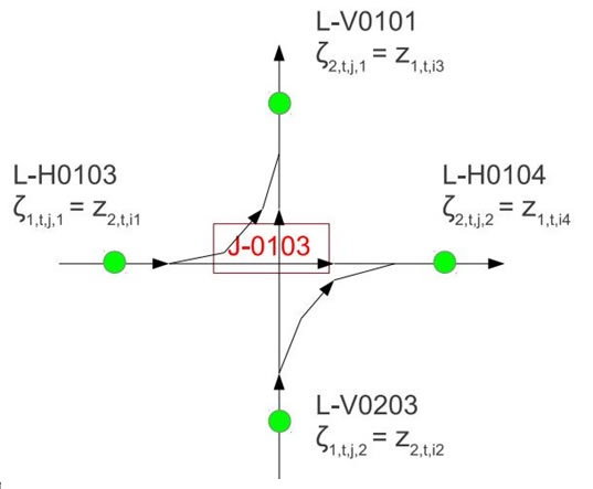
For the example in the figure, xt=xt,1:2 is a vector of length 2. At is a 2x2 turning matrix: At,i,1=logistic(xt,i), At,i,2=1-At,i,1. Sequential inference is applied on both state vector and unknown parameters, based on smooth functional approximation iterLap.
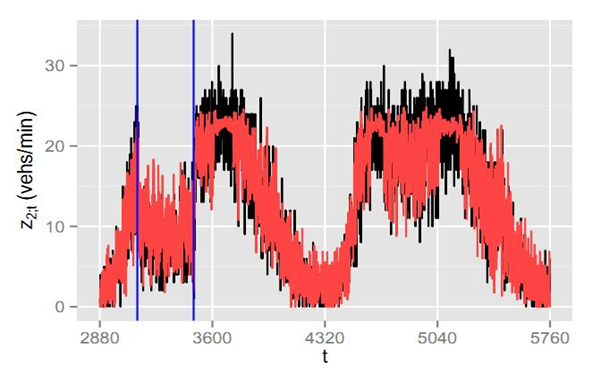
The results for junction J-0103 are as follows:
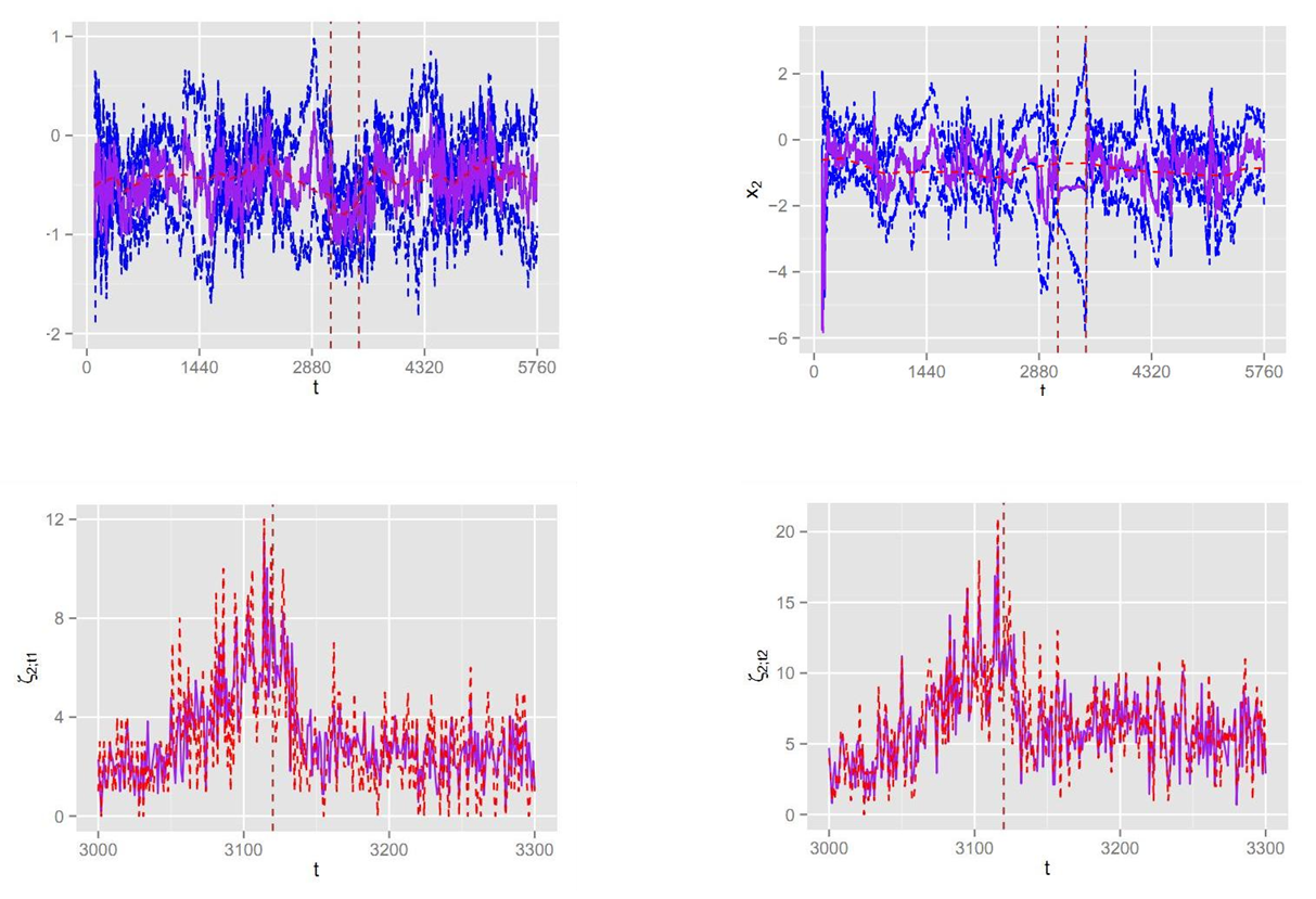
The top 2 graphs are a summary of the inferred distribution of xt. The blue and purple solid lines represents the mean and the mode of the distribution. The blue dashed lines mark the interval 2σ limits (roughly a 95% probability interval for xt). The red dashed lines represent the optimised series xt, using all data. The brown dashed vertical lines mark a duration when a traffic incident occurs. We see that the method has inferred values of xt that follow the optimal values quite closely, even during the traffic incident.
The bottom 2 graphs show the fit of ζζ2;t and ζ2;t to the data. Purple solid lines and red dashed lines are ζζ2;t and ζ2;t respectively. The brown dashed vertical lines mark the starting point of the traffic incident.
People
Tiep Mai, Simon P. Wilson, Bidisha Ghosh
Sponsors
![]()